


User Information
Area coverage
Table 1 and Table 2 provide a summary of the area coverage for enterprise budgets that were generated for this report (dryland- and irrigated regions). The source of data and collaborators are also presented. The collaborators are sincerely grateful for the interaction and assistance with data, knowledge and other inputs from each organisation, agribusiness and farmers.
| Area | Dryland crops | Source and Collaborators |
|---|---|---|
| Southern Cape | ||
| Caledon | Wheat, barley, canola, oats and lupins | Overberg Agri, GSA and BFAP |
| Bredasdorp | Wheat, barley, canola, oats and lupins | Overberg Agri, GSA and BFAP |
| Eastern Ruêns (high potential) | Wheat, barley, canola, oats and lupins | SSK, GSA and BFAP |
| Eastern Ruêns (normal potential) | Wheat, barley, canola, oats and lupins | SSK, GSA and BFAP |
| Eastern Ruêns (low potential) | Wheat, barley, canola, oats and lupins | SSK, GSA and BFAP |
| Western Cape | ||
| Southern Swartland | Wheat and canola | Kaap Agri, Overberg Agri, GSA and BFAP |
| Moorreesburg, Malmesbury and Porterville | Wheat, canola and oats | Kaap Agri, Overberg Agri, GSA and BFAP |
| Darling-vlakte – Hopefield | Wheat, canola and lupins | Kaap Agri, Overberg Agri, GSA and BFAP |
| Rooi Karoo | Wheat and canola | Kaap Agri, Overberg Agri, GSA and BFAP |
| Free State | ||
| Eastern Free State | Wheat | GSA / VKB / BFAP / Individual farmers |
| Central Free State | Wheat | GSA / SENWES / BFAP / Individual farmers |
| Area | Irrigated crops | Source and Collaborators |
|---|---|---|
| Northern Cape | ||
| GWK Area | Wheat, barley and canola | GWK, GSA and BFAP |
| Free State | ||
| Eastern Free State | Wheat | GSA / VKB / BFAP / Individual Farmers |
| Limpopo | ||
| Britz / Northam / Koedoeskop | Wheat and barley | GSA, Obaro and BFAP |
Yield assumptions
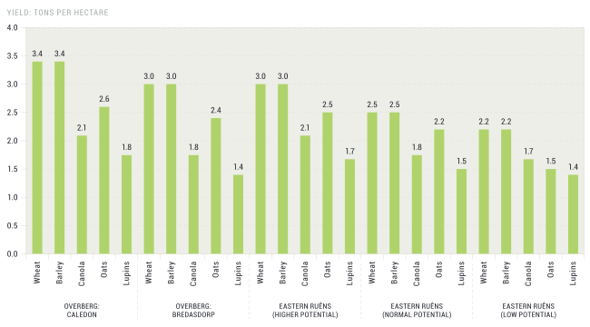
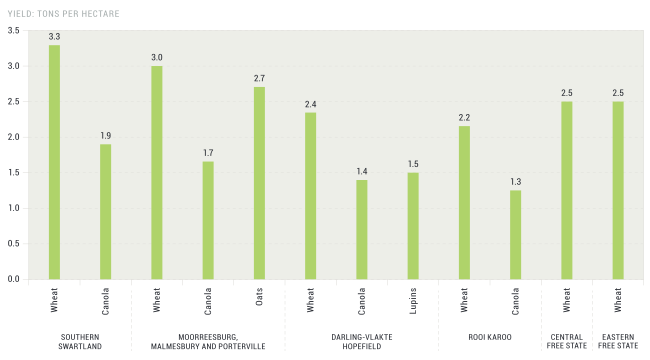
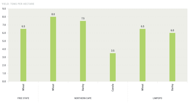
Table 1.3 illustrates descriptive statistics for yield trends over the period from 2005-2025 (2025 assumes trend yields). Figure 1.1 and Figure 1.2 reports the yield assumptions for dryland and irrigated crops. The yield assumptions represent target yields which were formulated in round table discussions and inputs provided by industry experts. These assumptions are re-evaluated and updated on a continuous basis. It is important to note that intra-regional variations will occur, and it is recommended that producers adjust their respective target yields based on their location and potential.
| Wheat: Winter area |
Wheat: Summer area |
Wheat: Irrigation |
Barley: Winter area |
Barley: Summer area |
Canola | |
|---|---|---|---|---|---|---|
| 2025 Assumed trend yields | 3.28 | 3.85 | 7.07 | 3.35 | 7.16 | 1.98 |
| Mean (2005-2025) | 2.70 | 3.18 | 6.35 | 2.89 | 6.48 | 1.46 |
| 3-year average (2022-2025) | 2.93 | 4.26 | 6.95 | 3.14 | 7.04 | 1.87 |
| 5-year average (2020-2025) | 3.10 | 4.42 | 6.85 | 3.27 | 7.01 | 1.95 |
| Min (2005-2025) | 1.80 | 1.53 | 5.27 | 1.95 | 5.19 | 0.90 |
| Median (2005-2025) | 2.68 | 2.80 | 6.43 | 3.12 | 6.61 | 1.35 |
| Max (2005-2025) | 3.50 | 5.05 | 7.15 | 3.95 | 7.16 | 2.25 |
Source: BFAP, 2025
Crop price assumptions
Annually, the Bureau for Food and Agricultural Policy (BFAP) presents an outlook of agricultural production, consumption, prices and trade in South Africa over a 10-year period. The information presented is based on assumptions about a range of economic, technological, environmental, political, institutional, and social factors. The outlook is generated by the BFAP system of models. A number of critical assumptions have to be made for baseline projections. One of the most important assumptions is that normal weather conditions will prevail in Southern Africa and around the world; therefore, yields grow constantly over the baseline as technology improves. Assumptions regarding the outlook of macroeconomic conditions are based on a combination of projections developed by the International Monetary Fund (IMF), the World Bank and the Bureau for Economic Research (BER) at Stellenbosch University. Baseline projections for world commodity markets were generated by FAPRI at the University of Missouri. Once the critical assumptions are captured in the BFAP system of models, the Outlook for all commodities is simulated within a closed system of equations. This implies that, for example, any shocks in the grain sector are transmitted to the livestock sector and vice versa. Therefore, for each commodity, important components of supply and demand are identified, after which an equilibrium is established through balance sheet principles by equalling total demand to total supply.
Table 1.4 illustrates the standard deduction from the base SAFEX or derived price as presented in Figure 1.3. Figure 1.3 illustrates the commodity price assumptions for wheat, barley, canola and oats that were used as base price for the winter crop budgets for the 2025 production season. The sensitivity analysis in the respective crop budgets makes provision for variation in price and yield and indicates the gross margin under each price and yield combination.
| Wheat | Barley | Canola | Oats | |
|---|---|---|---|---|
| SAFEX / Derived Price: 2025 | X | X (adjusted with price link for Southern Cape and Northern producing regions) |
X | X |
| – transport differential | X | X | X (for selective regions) |
Standard wheat transport differential + transport to processing facilities (estimate R200-R250 per ton) |
| – grade differential (BS, B1, B2, B3 and COW) | Based on historic averages; updated with new grading system | Assuming 10% of barley is downgraded to feed, and the remaining is delivered as malt barley | – | – |
| – silo, handling and administration costs | X | X | – | – |
| – statutory levies | X | X | X | X |
| + price premiums | BS calculated at 2% premium | X | Back payment calculated at 10% of derived price | – |
Source: BFAP, 2025
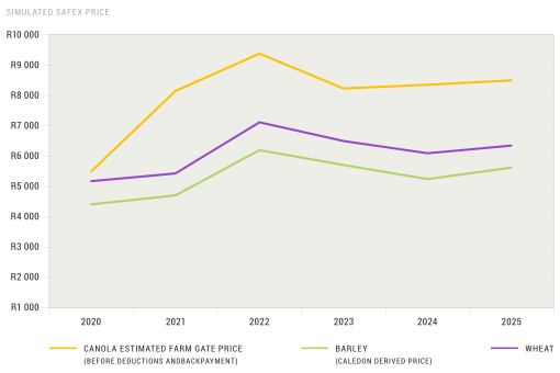
Figure 1.3 illustrates the projected local winter crop prices. South African prices reflect global price dynamics and are sensitive to exchange rate fluctuations. Global prices remain sensitive to the current geopolitical environment, with the tariff war creating further uncertainty. The US tariffs are likely to impact prices in the near future. Furthermore, the US stance on biofuel demand remains uncertain, affecting vegetable oil prices. Indonesia's biofuel policy timeline is unclear, but an extension has calmed markets. The B50 blend is planned for 2026.
The South African wheat tariff is expected to remain in place over the outlook period given current world price and production levels. Most crop production will rise in 2025, except for canola and sunflower. South America expects a record crop, lowering soybean prices. In the US, maize and winter wheat areas are projected to increase, while soybean area may decline slightly. EU conditions are fair, with canola production below potential but with an expected yield recovery, while wheat and barley production are projected to rise. The Black Sea region faces challenges with the Russia-Ukraine war, and Russia's wheat production is projected to decrease in 2025. Australia expects a strong winter crop, with a 16% year-over-year increase, especially for wheat.
The global and domestic environments are becoming increasingly complex, making it very difficult to navigate and manage future strategies. Multiple government changes in 2024 are creating policy uncertainty, which has implications for inflation and monetary policy, among others. The local GNU shows some signs of progress, indicating positive sentiments; however, stability concerns remain. Growing complexities and uncertainties in the trade environment increase compliance needs for exports and risks for export growth. Misinformation and disinformation are affecting decision-making. Sustainability is becoming increasingly important for policymakers, possibly creating additional compliance costs and affecting market access. Global growth prospects face negative risks, with a divergence in short-term growth prospects requiring fiscal sustainability.
Key input cost trends
Input costs are driven by multiple global and local factors, as a large share of inputs are imported. These factors include global supply and demand, industrial and trade policies, energy price dynamics, exchange rate, local manufacturing competitiveness, commodity markets, farmers' demand, logistics, and more.
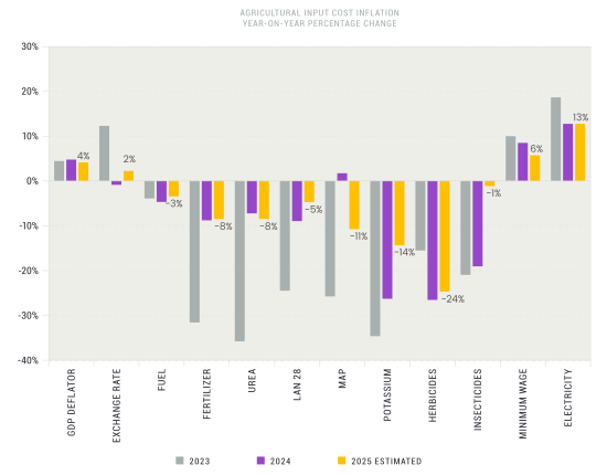
Figure 1.4 shows a calendar year-on-year percentage change for key agricultural inputs over the period from 2023 to 2025 (projected). In 2025, costs are generally expected to increase, while fertilizer and chemical prices are projected to decrease from the high levels observed in 2021 and 2022. Fertiliser and chemicals contributed roughly 40% to total direct costs for wheat, barley and canola, when considering data from 2018-2024.
Projections from the South African Reserve Bank indicate a modest expected GDP growth rate of 1.4% in 2025, driven by more stable electricity supply, monetary policy easing, and a return of investor and consumer confidence post-elections. However, the IMF recently revised its projection from 1.5% to just 1% due to the far-reaching impact of US tariffs. This could significantly affect the South African exchange rate.
Fuel costs are expected to decline slightly due to the global oil price drop following numerous tariff changes by US President Donald Trump. This may also affect fertiliser prices. The World Bank expects fertiliser costs to continue their downward trend in 2025 by 3%, but to start increasing again by 1% in 2026. The weighted domestic cost for fertilizer (a combination of nitrogen, phosphorus, and potassium) decreased by 9% in 2024 and is expected to continue declining at a rate of 8% in 2025. In 2025, urea, potassium, LAN (28), and MAP are expected to decline by 8%, 5%, 11%, and 14%, respectively. Plant protection chemicals have seen a significant decline over the last three years, with global herbicide prices decreasing by 26% and insecticides by 19% from 2023 to 2024. Global herbicides are further expected to decline by 24% in 2025, while insecticides are only expected to decrease by 1%. Electricity costs increased by 12.74%, according to NERSA’s approval.
While these downward trends are encouraging for producers, the cost of agricultural inputs remains significantly higher than pre-Russia-Ukraine war and pre-COVID-19 levels. For example, the local price of urea has dropped by nearly 50% from its peak in 2021-2022, yet it is still 59% higher compared to 2019.
Source: Grain SA and BFAP, updated April 2025
Methodology, approach and definitions
- A standard operating procedure was used across all crops and regions for generating the cost and income budgets for the 2025 winter production season.
- Deterministic or target yields are based on industry discussions which refer to a yield that should be obtained given a normal production season with normal weather in the respective agro-ecological production regions.
- The farm gate price for each crop is calculated by deducting transport differential, grade differential, handling fees, commission and levies (statutory for seed breeding and technology) from the BFAP simulated SAFEX price and adding price premiums, as discussed in Table 1.4.
- The gross production value is then calculated by multiplying the yield with the farm gate price.
- The direct costs are calculated by multiplying the cost per unit by the estimated quantity of input use or application rate.
- For the majority of the crops, it is assumed that own machinery is used, except for speciality operations that are coupled with economies of scale. In such cases, a contracting cost item is allocated.
- In the Western Cape, provision was made for fire and SASRIA crop insurance, and in the northern parts of South Africa, provision was made for hail insurance.
- Fertiliser and lime application will vary significantly in regions and across crops, however, an attempt was made to follow a standardised approach across the regions. Micro-elements and foliar feed for selective crops are included in the total fertiliser cost.
- The price for fertiliser nutrients (N, P & K) was calculated by using a weighted approach that accounts for 1) variation in discounts received from suppliers and 2) the time period when fertilisers were purchased.
- Fuel consumption is based on the prevalence production system in each region.
- For plant protection, herbicide, insecticide and fungicides are accounted for based on interaction with industry experts and producers. For instance, in certain regions provision was made for fungicide sprays, but for others where the practice is not common, fungicides were excluded from plant protection costs.
- Repairs and maintenance costs are calculated based on the production system operations and were consulted with industry experts and producers.
- An average seed price across various seed companies was used for calculating the cost of seed. The cost of seed per hectare is calculated by multiplying the cost per unit (either kilograms or plant population) by the application rate per hectare. For selective crops, seed treatment was included where relevant. For wheat and barley, the seed application rate was sub-divided according to own and purchased seed. For own seed use, a cost is allocated which is based on a realistic crop price (hence, opportunity cost) and seed preparation costs such as sifting and treatment.
- For irrigated crops, the cost of water and electricity is calculated according to typical irrigation application rates at their respective regional costs per millimetre water applied throughout a season. For instance, variations will occur in the cost for water in areas where predominantly boreholes are used compared to irrigation/water scheme areas.
- The gross margin was calculated by subtracting the direct cost from the gross production value.
- Overhead costs and production interest are not accounted for in the enterprise budgets.